|
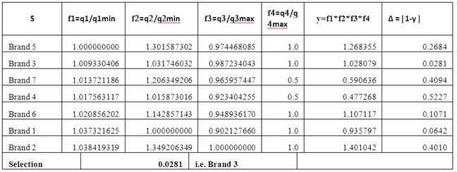
Abstract – In Industrial Buying, especially in government purchasing, the procedure adopted is to use only the quoted price as the determinant in arriving at the ranking among a batch of suppliers who have participated in a tender inquiry and identify the lowest price supplier to place orders on them. The total cost of ownership of the item which would include costs such as the running costs, maintenance costs during the useful life are not factored in evaluating the offers, though this method is adopted in large value purchases such as in capital expenditure. While computing the total cost of ownership for each offer would be cumbersome, a quick method would be the ratio method, in which the parameters of evaluation which would include the price are compared inter-se with the best of parameters identified from among the offers received. The authors present a case-study in this paper demonstrating the simplicity of this method for preparing a comparative chart which can be used to select the best supplier for awarding an order. Keywords— bench-marking, optimal buying I. INTRODUCTION In the world of supply chain management, in the procurement of goods and services, purchasing decisions are normally made based on the prices that are quoted by the suppliers. The tendency is to buy from the lowest cost quote, subject to of course the offer meeting the (technical) specifications, needs and requirements of the buyer. Apart from the price, commercial terms also influence the buying decision – such as the delivery periods offered, the payment terms, the guarantees / warranties and such others. However, when the buying is for capital goods, the approach adopted is to calculate the total cost of ownership (TCO) by computing the cost of owning the machine through its life-time (usually referred to a Life Cycle Costing [LCC]). For example when investing in a lathe or a diesel generator set, the total costs would be arrived at by adding to the price of purchase, the running costs that would be incurred by way of power / fuel, costs charged by the original equipment manufacturer (O.E.M) for periodic maintenance, the replacement cycle of the parts of the equipment during its productive life and the projected costs thereof. The total cost so arrived for each supplier in a batch of acceptable offers is then compared. The lowest cost in such a computation would be the winning price. Some of the buyers, instead of resorting to such a calculation, specify a baseline requirement covering key parameters. Penalties are added, where the offer exceeds the datum line. The price arrived after taking into consideration the load-factors are then compared to fix the lowest acceptable price. The third method (illustrated here) is bench-marking each of the offer received. Parameters are compared inter-se with respect to the best of the lot. After normalizing each parameter with respect to the best of the lot, a composite score is arrived at by combining the parameters and the selection is made. The offer that is nearest to the ideal is selected by the buyer. The advantage of this method is it is simple. Even a high-school student can do the arithmetic and would be able to identify the optimal buy. II. BENCHMARKING METHODOLOGY A. The Problem First let us turn to Table 1. Suffice it now to explain that the first column represents the various offers in the hands of the buyer. q1 to q4 are the determinants of the buy, with q1 representing the price of the material. The last column R gives the price ranking of the offers without considering the impact of the other factors viz. q2, q3, and q4. L1 represents the first lowest, L2 the next higher and so on. The question that now arises is that – how to factor the impact of q2, q3, and q4 along with the price q1 and determines the best buy. For sake of lucidity, we shall now define S and the thetas based on a simple but real life (old) case-study. 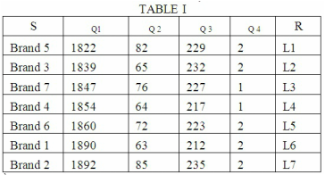 Let S be the purchase of ceiling fans. Let us consider a large buy of say 2500 ceiling fans for a new office complex that is coming up. At current market price, the architect estimates the likely expend on the ceiling fans as Rs. 50 Lacs. q2 is the power consumed by the fan, expressed in watts, q3 is the air delivery of the fan, measured in cubic meters per minute (CMM), and q4 is the number of bearings – 1 representing a fan with a single bush bearing and 2 representing a fan with double ball bearing. The requirement of the buyer is to identify the supplier who can supply the fan at: The lowest cost, With the lowest power consumption, and The highest air delivery. The fan with double ball bearing is considered as technologically superior to a fan with a single bush bearing. After getting the quotes, each Supplier had to supply a ‘test’ fan for evaluation by the Buyer. The buyer then conducted his own tests in his premises and the results that he got are that which are tabulated in TABLE – I. B. Analysis and Solution In the first step the received data are analyzed. It is evident that the prices are randomly varying between Rs. 1800/_ and Rs. 1900/_. Similarly the power consumed varies between 60W and 85W and the air delivery between 210 CMM and 235 CMM. In the second step the lowest value in each column is identified qmn-min. Each entry in a cell qmn is divided by the qmin of that column. The resulting fraction is then filled in each cell. The result with the fractions filled is given in Table-2 as fmn. Across each row the fractions are multiplied and the result is designated as: y. (Column 6 of TABLE – 2). The absolute value of the difference of y with respect to Unity is computed as Δ and filled in. (column 7 of TABLE 2). The minimum of Δ is the selection of the best purchase for the buyer. q1 = Price quoted by the Supplier in Indian Rupees. q2 = Power consumption measured in Watts q3 = Air delivery in cubic meters per minute (CMM) q4 = Number and type of Bearings R = Rank C. Explanation
Once the optimal fan was selected, the purchase decision maker, embarked on the following course of action.
 IV. CONCLUSION
By adopting this simple bench-marking approach (presented here), the buyer was able to select the near ideal ceiling fan for his use. The approach taken by the buyer was simple and did not require any complicated calculations. FURTHER READING [1] P. Glucha and H. Baumann, “The life cycle costing (LCC) approach: a conceptual discussion of its usefulness for environmental decision-making,” Building and Environment 39 (2004) pp. 571 – 580, October 2003 [2] B.S. Dhillon, Life Cycle Costing, Techniques Models and Applications, Gordon and Breach Science Publishers, 1989 [3] J. Emblemsvag, Life-Cycle Costing: Using Activity-Based Costing and Monte Carlo Methods to Manage Future Costs and Risks, John Wiley & Sons, 2003 [4] M. Devi, Total Cost Of Ownership - An Introduction, ICFAI University Press, 2005 [5] B. Andersen, P.G. Pettersen, Benchmarking Handbook, Springer Science & Business Media, 1995 [6] M. Zairi, Effective Benchmarking, Springer Science & Business Media, 1996 [7] T.Stapenhurst, The Benchmarking Book, Routledge, 2009 [8] R. Monczka, R. Handfield, L. Giunipero and J. Patterson, Purchasing and Supply Chain Management, Cengage Learning, 2008 [9] V.H. Pooler, Purchasing and Supply Management: Creating the Vision, Springer Science & Business Media, 1997 [10] P. Gopalakrishnan and A. Haleem, Handbook of Materials Management, PHI Learning Pvt. Ltd., 2015 [11] L. Lee and D.W. Dobler, Purchasing and Materials Management, McGraw-Hill Inc.,US; 3Rev Ed, 1977
0 Comments
|
AuthorCyril R. Fernandez ArchivesCategories |
Cyril F blogs
-
Blog Home
- Text of Speech given in an Engineering College
- A short lit survey on Work-Life Balance.
- A short lit survey on Work-Life Balance.
- Bull whip effect
- A Pilot Study of Impact of Religious TV channels on households in a Vellore suburb
- Should Price be the only criterion in buying? - A Case Study
- Cultural Hybridization in an Industrial Township – A Case Study
- A Literature Survey of the Internet Resources on Deconstruction and Literature
- A case-Study on a performance evaluation system of officers in a Public Sector Undertaking in India.
- Concept of an automated purchase
- Pitfalls in Supplier Development - A Case Study
- English Literature in the Digital Era
- A Model for measuring Supplier Satisfaction
- Impact of Social Networking Sites (SNS) on Indian youth
- Impact of Social Networking Sites on today’s youth
- Industrial Marketing in the digital era: An Indian perspective
- About
- Contact
 RSS Feed
