|
Introduction On input (raw) material supply side, Inventory may be explained as the sum of the value of goods physically available in the Stores plus that which are in transit from the suppliers plus the materials that are part-processed and available either in the shop-floor or with the sub-contractors (called work-in-process). Extensive literature is available on Inventory and Inventory management under topics like – Purchasing Management, Materials Management, Supply Chain management and Logistics management. Therefore the authors propose not to dwell here in detail upon the fundamentals of Inventory and Inventory management except for the brief (and perhaps a superfluous) touch-down on Inventory, but to present in this article a simple schema for automating a small part of an organization’s inventory management. As it is well known, Inventory is a buffer to ensure continuous and uninterrupted production in a manufacturing organization. It is also a well known fact that next to the fixed assets, Inventory is the largest investment for any organization. But Inventory is a burden-cost, since the Inventory is a dead asset funded by expensive working-capital - financed by higher interest bearing borrowings. Therefore there is a pressing need for a manufacturing organization to optimize the inventory – balancing the need to keep it at the lowest level (to reduce the inventory carrying costs) and at the same time providing a buffer to ensure uninterrupted production. The buffer of inventory is essential to cover the vagaries of not only the production rate in the organization (arising out of customer orders) but also to cover the uncertainties in the input side of the supply chain. In the Indian context, the supply side uncertainties are exacerbated – suppliers are known for late and delayed shipments (which in many cases pervades throughout the supply chain – where even if a delay occurs in one link in the chain the cascading effect has a telling impact across the users – a reverse bull-whip effect in fact.) This means that industries without a dedicated set of suppliers need to rely largely on their inventory for ensuring unhindered production, to gain customer satisfaction. Inventory is also required to balance the incidences of incoming material rejections. Though the quality consciousness of the Indian suppliers is growing there still lingers the threat of incoming material rejections on account of the material being defective or not meeting the ordered specifications. Organizations do try to mitigate this threat by increasing their quality control efforts by resorting to at-source inspection prior to dispatch. However this adds to the costs of quality which in turn is an avoidable, unnecessary and invisible add-on cost which the end customer has to pay for. Where there is a dedicated and committed set of suppliers (see the manufacturers of cars like Maruti etc.) who support of the organization through mechanisms like just-in-time supply or vendor managed inventory (VMI), the inventory levels are pared down in the buying organization as the inventory burden is now spread across the chain. Just in time inventory does not mean absolute zero inventory but connotes a minimalist level of inventory maintenance to cover any hiccups that may happen on the production line or to cover the blips in the supply chain. The impact of inventory on the customer satisfaction and on the financial results (profitability) is so high that today Inventory has become a subject of major concern to the management. In these days of difficult business the management-thought today is to see inventory as a financial liability (locking up the scarce resource of money) and not as a current ‘asset’. Sophisticated tools are employed by organizations for inventory management. With high investments in Information technology, companies are leveraging the ICT route for optimal inventory management. Especially where the manufacture model is ‘make-to-stock’ with a continuous production line, the utilization of software tools for inventory management is high and is also cost-effective. In the ‘make-to-order’ model higher levels of sophistication may not have been achieved for inventory management because of the range and variety of the input materials for each customer order. Even in this type of operations, there would be common items which would be used across various customer orders. Such items would be ideally amenable for inventory control and management. The authors submit here an automation tool for such a model. System Design The start point would be to identify the stock-items which are required and used across all or most of the customer orders. (Identifying the common denominators). For example an organization involved in the manufacture of engineered goods may be using specific raw material steel (plates, sheets and structural) across various customer orders. Again for example in an organization, 6 mm steel plate or a 1.6 mm stainless steel sheet or Channel 400 x 100 mm may be common item used in most or all of its manufactured products. These items could constitute high cost, high consumption input items. At the other end of the spectrum there may be items like a Hexagonal Screw and Nut set which would be high consumption and low cost item. The underlying feature of these two extremes (in terms of costs) is the consumption pattern – being high. A history analysis can be deployed to study the consumption pattern which would easily identify the high consumption items. One of the standard analytic tool that can be effectively employed is the Pareto Analysis (also popularly termed as the ABC analysis). ABC analysis by velocity of the materials issued from the Stores can be used to identify the “C” class items easily – the high consumption and low value items. The analysis can be used to identify the other high consumption items also. In this particular case study the authors have selected those items which were issued 50 times and above in a financial year for the selective inventory control. Within the database of the material category a sub-data base was developed by flagging those having high consumption. This exercise was done on a horizon of the past three years. (The authors recommend that this data base may be updated on an annual basis to mark the high consumption items – which would be stocked and for which the replenishment purchase requisitions generation can be automated as described in the following sections.). This data base is designated as STK_ITEM_FOR_CONT. The second step is to calculate the lead time (lead time analysis) for each of the stocked item selected for control. Analysis of the supply lead time is done by trawling through the supply data of the selected items. The data analysis is done for the past 5 years and the modal value of the lead-time is computed. The lead-times so computed are compiled into a database named as L_TIME. The L_TIME data base is always kept current by updating it for every event of supply made for the material under control. For every supply made and accounted for in the stores the time in number of days elapsed between the order date and the supply date is calculated and pushed into the SUPP_HIST data base. 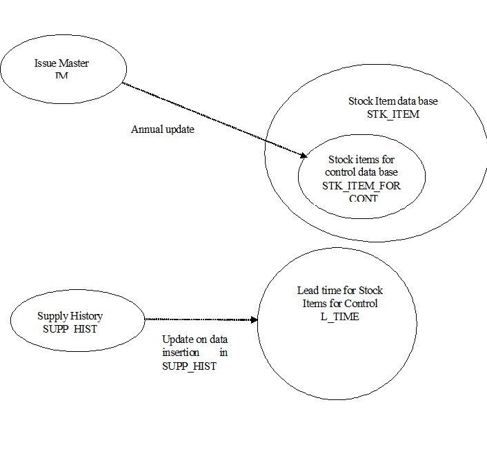 The Supplier history is the database where this information is stored. The transactions of the materials are stored in the IM (Issue-Master) data base. Coding the program Platform: The test system was developed on Oracle 10g platform The proposed inventory control / automated purchase requisition generation is modeled on the fixed period review methodology. The review period (r) is set as one (1) week. All time periods would be measured in weeks. The start point would be initializing the system parameters. The steps advocated for these are as follows: Initialize Day = Monday {The review will be done on every Monday at 06:00 hrs by programming the system to run the software at this appointed time} Review period r = 1 week Service level Z = 1.3 Lead time consumption (L) = 0 Safety Stock (SS) = 0 Base Stock (B) = 0 Normal Indent Quantity (NQ) = 0 Emergency Indent Quantity (EQ) = 0 Select Stock for Control item Lead time for the Stock for Control item from the L_Time Table. Calculate Lead time consumption (L) (L is the quantity consumed during L_Time picked from the Issue Master (IM)) Mean of the lead time consumption m Consumption during the lead time and the review time Lt Standard deviation of the consumption during lead time s Safety Stock (SS) Base Stock (B) {e.g.: If the lead time is 6 weeks and the issue data shows the consumption in the immediate past 6 weeks measured in terms of the stock keeping units (sku) as: Week 6: 120, Week 5: 30, Week 4: 80, Week 3: 75, Week 2: 62 and Week 1: 90 Units then the average consumption in the lead time period is computed as MEAN(120,30,80,75,62,95). (Note: In the instance case the mean value m would be 77) Total consumption Lt is calculated as the product of the average consumption with the sum of the lead time and the review time. (Note: In our case with the review period ‘r’ being 1 and the lead-time being 6 the consumption is calculated as m (r+L). This works out as 77*7 = 539 sku). The standard deviation during the lead time is calculated as STDEV(120,30,80,75,62,95). (Note: In the instance case it works out to 30 sku. The value computed is rounded off to the nearest sku). The safety stock is found as the product of the adopted Service level, the Standard deviation of consumption during the lead time and the square root of the lead time and the review time. SS = Z * s * Sqrt (r+L) (In our case it would be = 1.30 * 30 * SQRT (1 + 6) which yields a result of 103 sku). The SS so calculated is converted to the consumption multiple of a standard product of the organization. If the organization manufactures three different items which are to be supplied together for a single customer and the customer order would stand fulfilled only when the three sub-products supply is completed together and if the (raw) material under reference is consumed across all the three products and for a typical order of the three items, the quantum of the raw material required is 125 sku then the safety stock is kept as 125. In the event the requirement is only 95 then the SS would be kept at 95. The SS level would be essentially determined by the cycle time of a given typical order execution. The SS can be computed in terms of one unit of customer order or multiple units of customer orders. The decision maker should factor the lead time of supply and the lead time of manufacture for determining his / her SS. If the manufacture lead time is less than the supply lead time, then the SS should be fixed at the least equal to lead time consumption (including the review period) but to err on the side of caution the authors recommend that the materials manager should prefer to keep the SS at a higher level - for eg as 1.5 or 1.2 times the computed SS. We leave it to the confidence level of the materials manager on the competency, efficiency and the effectiveness of the supplier/s of the material under reference. The Base stock B is computed as B = SS + Lt (In our example if SS is fixed as 120 then B = 120 + 539, which is 659. The result obtained can be rounded off in terms of the minimum lot of supply (if it so exists). If for the supplier the minimum lot of supplies is in multiples of 100s, then the Base Stock would be fixed as 700 sku by the materials manager). The software can be programmed to calculate the SS and B from the data available in the data base. Once the SS and B are fixed the periodic review system can be implemented as an auto-tool for generating purchase requisitions. Large organizations have exclusive specialist material planning department responsible for generating purchase requisitions. The manpower deployed on planning for such high volume transaction items can be reduced by resorting to developing an automated software on the basis of the approach outlined in this article. Then with minimum human intervention the inventory of such items can easily be monitored and managed using the outlined proposal. Once the SS is fixed for each of the sku, the software is programmed to cycle through the lines of codes every week on the appointed day. (In our case, it is Monday) The logic for the auto-indent generation is as follows: The steps are shown for one sku and the program is made so that the computation is done for all the skus in the master maintained by cycling through it for auto-indent generation. The Base Stock (B) is calculated as above. Compare the Base Stock (B) with the actual inventory (A) in hand (on the day of the computation). If A > B The system would not trigger any action but would cycle back to the next sku If SS > A Then two actions would be triggered by the system program:
A purchase requisition would be generated for quantity (B-A). Based on the auto-requisition generated by the system, the purchasing group can initiate its procurement action. Where the organization has running or a rate contract with the supplier of the sku, the system can be programmed to send an e-mail order directly to the supplier with the demand quantity. Testing (Inventory Simulation) The program was tested with historical data as a simulation study. The simulation run was made for 250 Monday statistics for a specific sku and was compared with the actual levels of inventory as available in the database. While real-life saw stock-out situations were noticed, it was seen that the simulation run eliminates the stock-out situations. There were instances where the simulation run threw up emergency indents but with the auto-indenting system, but there were no stock-out instances. The month to month average levels of inventory was reduced but the number of ordering episodes went up. Conclusion This planning software delivers! This simple mechanism of automating the purchase requisition delivers maximum advantages. For one, it reduces the human efforts. The released manpower resources can be redeployed elsewhere, more profitably, within the organization or can be better employed for a more effective inventory control – as in controlling the “A” category items. (High Value- Low consumption, Customer specific raw material input). It reduces the average inventory levels freeing up the scarce resource of money locked up as inventory. There is a tight knitting of the demand forecast as it strongly coupled with the actual inventory movement. The shop-floor demand data and current inventory status get strongly tied with the periodic (weekly) automated review system. (Information Integration) The work-flow coordination between the planning and execution (purchasing) becomes automated and streamlined and delivers efficiency. The demands become more accurate infallible to human failings and timely, consequently leading to cost efficiency. And finally the quality of the demand gets improved. References: Supply Chain Management : Texts and Cases by V.V. Sople Designing and Managing Supply Chain: Concepts, Strategies and case Studies by Shimchi-Levi, Kaminski and others Decision Flow chart for auto-indenting 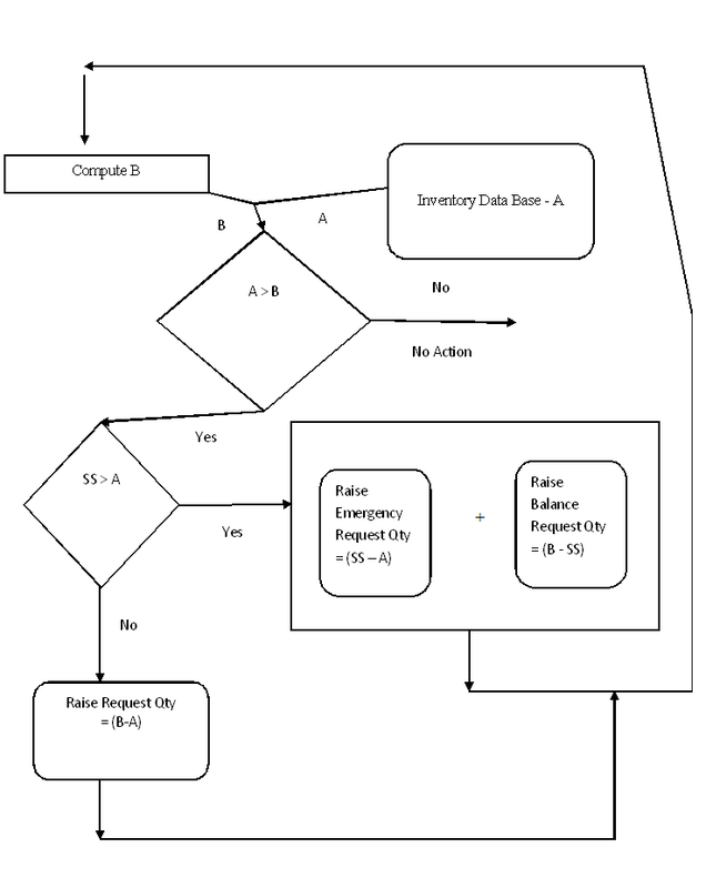 (This article is prepared by Cyril R. Fernandez General Manager / Materials Management, BHEL, Ranipet jointly with Shri. S. Krishnamoorthy Engineer / MM Systems, BHEL, Ranipet) 
0 Comments
|
AuthorCyril Fernandez and ArchivesCategories |
Cyril F blogs
-
Blog Home
- Text of Speech given in an Engineering College
- A short lit survey on Work-Life Balance.
- A short lit survey on Work-Life Balance.
- Bull whip effect
- A Pilot Study of Impact of Religious TV channels on households in a Vellore suburb
- Should Price be the only criterion in buying? - A Case Study
- Cultural Hybridization in an Industrial Township – A Case Study
- A Literature Survey of the Internet Resources on Deconstruction and Literature
- A case-Study on a performance evaluation system of officers in a Public Sector Undertaking in India.
- Concept of an automated purchase
- Pitfalls in Supplier Development - A Case Study
- English Literature in the Digital Era
- A Model for measuring Supplier Satisfaction
- Impact of Social Networking Sites (SNS) on Indian youth
- Impact of Social Networking Sites on today’s youth
- Industrial Marketing in the digital era: An Indian perspective
- About
- Contact
 RSS Feed
